A / ONE-PARAMETER CROSSINGN=4 CHAIN
A line crosses the branch point.The gap closes at γEP; non-adiabatic transfer and gain/loss decide the final mode.
01 A DYNAMICAL FIELD NOTE
An exceptional point is more than a spectral crossing. Modes coalesce, the gap closes, and time evolution becomes sensitive to how the system moves through parameter space.
WATCH THE EXPLAINER
A narrated field note on mode coalescence, crossing versus encircling, and the N=4 slow-ramp result. The loop is an illustrative two-level model; the computed chain result is a separate one-parameter crossing.
02 THE SINGULAR POINT
An ordinary degeneracy brings eigenvalues together while their eigenvectors can remain distinct. At an exceptional point, eigenvalues and eigenvectors coalesce. The matrix becomes defective, and its local eigenvalue branches typically have a square-root form.
The branch point sits at z = 0. One loop around it exchanges the analytic eigenvalue sheets.
The normal form is an illustrative two-level model. The N=4 XXZ results below come from a separate, one-parameter chain calculation.
03 PATH-DEPENDENT EVOLUTION
The spectrum tells you where the modes are. The trajectory and the elapsed time determine which state survives.
LIVE TWO-LEVEL LOOP
Integrate i∂tψ = H(z(t))ψ around z=0. This is a pedagogical local model—not the N=4 chain.
Move the progress slider or play the loop. Endpoint weights are coordinates in a nonorthogonal right-eigenvector basis, not probabilities.
Illustrative parameters: H(z) = [[0, 1], [z, 0]], z(t) = 0.2 exp(±2πit/T). Positive angle is counterclockwise. A single circuit returns to the same matrix but can return on a different mode branch.
04 THE COMPUTED CHAIN
A separate, numerical test of a one-parameter crossing—no loop around the EP.
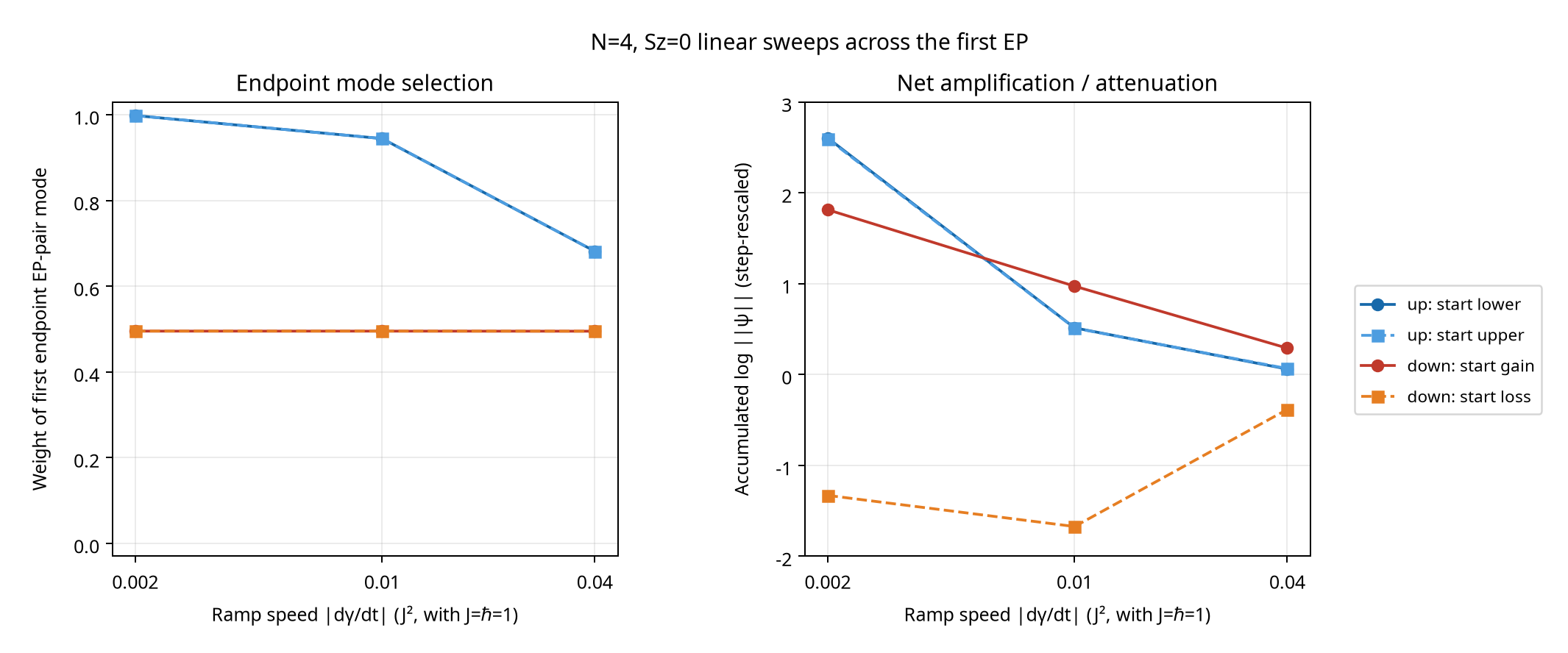
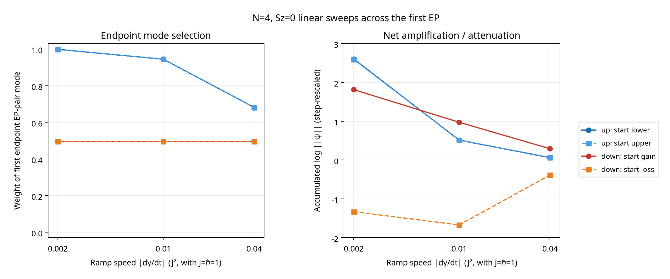
For a ramp from γEP−0.04 to γEP+0.04, both initial states increasingly finish in the positive-imaginary-energy mode. At speed 0.002, its right-eigenbasis coordinate weight is 99.83%.
Downward ramps end near 49.5/50.5 in the lower/upper pair coordinates. The final state still depends strongly on the starting branch and ramp speed; equal coordinates do not mean identical states.
Below the EP, the lower real branch continues to the positive-imaginary branch; the upper continues to the negative-imaginary one.
Non-adiabatic transfer plus differential gain/loss can override that branch mapping. In the slow upward ramp, both starts select gain.
The chain result crosses a one-dimensional threshold. Clockwise/counterclockwise behavior belongs to a separate encircling protocol.
05 THE SHORT VERSION
The N=4 case has a second-order Jordan block in the Sz=0 sector.
Crossing and encircling are different protocols. Direction and speed can change the surviving mode.
Report the normalization convention alongside any non-Hermitian “population” or mode weight.
EP = exceptional point · γ = staggered imaginary-field strength · z = local complex control parameter · CW/CCW = clockwise/counterclockwise · gain/loss = positive/negative Im(E) for i∂tψ = Hψ.
06 OPEN RECORD
The numerical chain result is separate from the illustrative two-level loop. Download the source and data used for the N=4 crossing analysis.
Place both Python files in the same directory. With Python 3, NumPy, and Matplotlib installed, run:
python -m pip install numpy matplotlib
python phase_ii_ep_dynamics.py
The script writes the CSV and plot beside itself. The logged coordinates are right-eigenbasis diagnostics, not Born probabilities.
PHASE II-F / STATUSThe EP location, Jordan structure, and dynamics results presented here were computed from operator definitions and are reproducible from the artifacts linked below. Phase II-F activation and EP-shift results are separate and remain unreproducible from the accessible public record pending recovery of the original source code.